 |
Bartek Wilczyński and Norbert Dojer
This short tutorial presents the most common possible uses of the BNfinder software. The first part of this tutorial is devoted to presenting possible options of the software an the input files on simplistic, synthetic examples. In the second part, we provide more realistic examples taken from published studies of data for inferring dynamic and static networks.
In this tutorial, we will assume that you are using the standalone BNfinder application as downloaded from http://bioputer.mimuw.edu.pl/software/bnf, however if you want, you can also try out these examples with our webserver at http://bioputer.mimuw.edu.pl/BIAS/BNFinder.
If you have any questions regarding this document or the described software, please contact us: bartek@mimuw.edu.pl or dojer@mimuw.edu.pl
| |
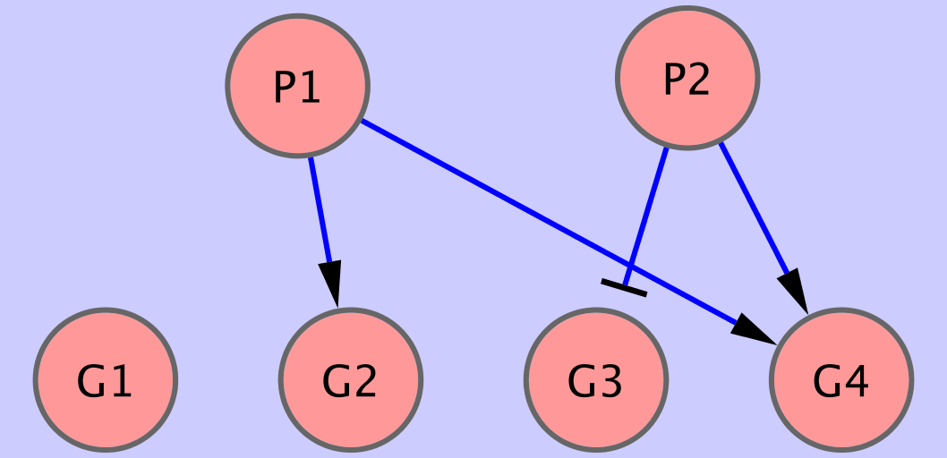
The first example shows how to use BNfinder to learn a simple static
Bayesian network. Let us imagine that we are analysisng cells under
two conditions ![]() and
and ![]() and that we are interested whether any of
the four genes:
and that we are interested whether any of
the four genes: ![]() are responding to these conditions. We
assume that the true network is depicted in Fig 1, i.e.
are responding to these conditions. We
assume that the true network is depicted in Fig 1, i.e.
We have collected 100 datapoints from this network, each consisting of both the state of conditions and the discrete state of expression of the genes. You can download the input file here data/input1.txt.
If you open the file in a text editor, please note that the first line contains the information on the assumed structure:
#regulators P1 P2This represents the fact, that we assume that genes (
You can try to run BNfinder on this file:
bnf -e input1.txt -n output1.sif -vand you will see, that the network topology is reconstructed properly. Also the orientation of the regulatory interactions is inferred properly as you can see in the output file data/output1.sif.
You can also try to see whether the optimal network is representative for a larger set of possible suboptimal networks:
bnf -e input1.txt -n output1w.sif -v -i 5 -txt output1.txtThis time, in the output file (data/output1w.sif), the edge labels represent the relative weights of different edges. In the file data/output1.txt, we can find the originally computed weights for all considered suboptimal sets of parents for all genes.
We can also try to analyze the data for this network without discretization: data/input2.txt. In this case we need another directive to indicate that some of the dataseries are continuous:
#continuous G1 G2 G3 G4
Again if we run BNfinder on this data,
bnf -e input2.txt -n output2.sif -vwe can verify, that the output file contains correct information data/output2.sif.
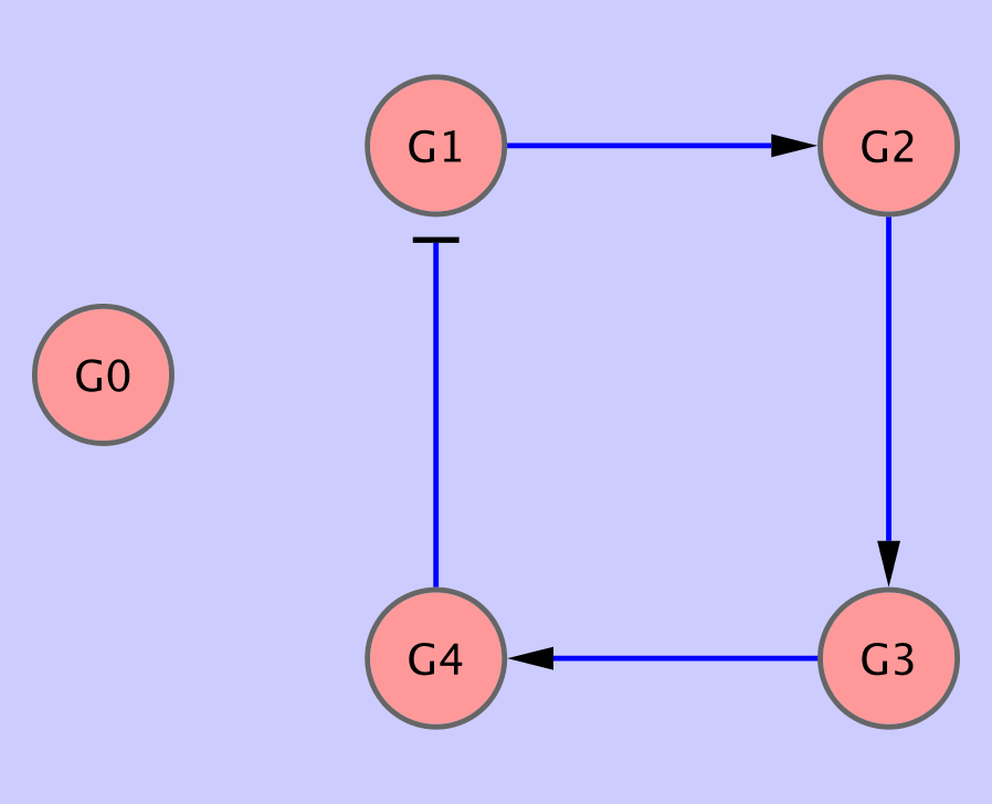
BNfinder can be used also to infer dynamic Bayesian networks from time series data. In this case it is not necessary to specify the regulators sets, because DBNs, unlike static networks do not need to be acyclic.
In the first dataset: data/input3.txt, we have 1 serie of 20 consecutive measurements of gene expression from gene network depicted in Fig. 2.
 |
If we run BNfinder on this data:
bnf -e input3.txt -n output3.sif -vWe can see that the program was unable to correctly reconstruct all the edges. Again, if we look at the statistics of edge occurences in suboptimal networks,
bnf -e input3.txt -n output3.sif -v -i 10 -txt output3.txtwe can see that the correct edges are the most commonly occuring ones, but they score lower than empty parent sets.
In this case we can show how perturbational data can be integrated into this framework. We have collected gene expression from 5 time-series containing one single gene knockout for each of the genes: data/input4.txt. The perturbations are noted by including the following lines in the preamble of the data file:
#perturbed EXP1 G1
#perturbed EXP2 G2
#perturbed EXP3 G3
#perturbed EXP4 G4
#perturbed EXP5 G0
If we run BNfinder on the perurbed data, we can see that all the edges are reconstructed with high confidence.
bnf -e input4.txt -n output4.sif -v -i 10 -txt output4.txt
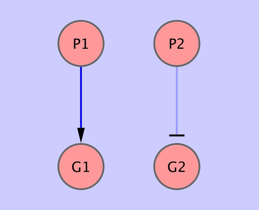 |
bnf -e input5.txt -n output5.sif -v -i 10 -t output5.txtwe can see that the program is unable to recover the
#prioredge G2 0.33 P2 P1we can see the edge appearing in the result as expected (see data/input6a.txt):
bnf -e input6a.txt -n output6a.sif -v -i 10 -t output6a.txt
Similarly, if we expect, that in general gene response to condition ![]() is weaker, we may modify the prior probability of the condition
is weaker, we may modify the prior probability of the condition ![]() to be a regulator:
to be a regulator:
#priorvert 0.33 P2
The result of running BNFinder with this input (data/input6b.txt) is very similar to the previous one:
bnf -e input6b.txt -n output6b.sif -v -i 10 -t output6b.txt
In this section, we present two more realistic examples of published datasets used for inference of Bayesian networks. The first one consists of measurements of states of protein signalling network under different perturbations [1]. It's been used to infer causal relationships in the form of static Bayesian network.
The second dataset comes from documentation of the Banjo package [2] which can be downloaded from (1]. We took the data from the article, and transformed it into the format suitable for BNfinder. We also needed to specify several properties of the data in the preamble of the file data/sachs.inp
 |
Firstly, we needed to specify that the data are continuous measurements:
#continuous praf pmek plcg PIP2 PIP3 p44/42 pakts473 PKA PKC P38 pjnk
Then, we needed to specify the expected layer structure of the signalling pathway we are studying:
#regulators plcg
#regulators PIP3
#regulators PIP2
#regulators PKC
#regulators PKA
#regulators praf
#regulators pjnk pmek P38
#regulators p44/42
#regulators pakts473
Then we needed to specify which of the proteins are affected by different perturbations.
#perturbed cd3cd28psitect_0 PIP2
#perturbed cd3cd28psitect_1 PIP2
#perturbed cd3cd28psitect_2 PIP2
...
#perturbed cd3cd28g0076_0 PKC
#perturbed cd3cd28g0076_1 PKC
#perturbed cd3cd28g0076_2 PKC
...
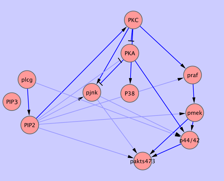
When we finally run the BNfinder:
bnf -e sachs.inp -n sach.sif -vWe obtain the network presented in Fig. 4. As we can see, the topology is quite consistent with the literature data. Out of 17 expected edges, BNfinder recovers 11 correctly.
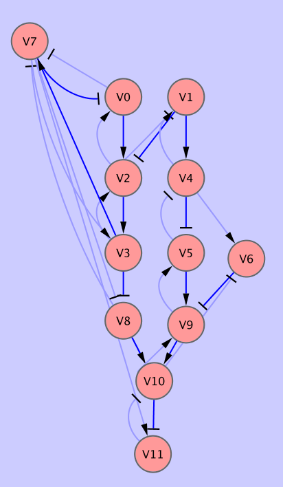
This is a dataset of substantial size which is used [3] to assess the performance of our inference algorithm. The input dataset (data/input7.txt) consists of 2000 measurments of 20 variables nd it takes approximately 3 hours to compute it on a modern PC (2.4Ghz Intel Core 2 duo).
We can run BNfinder with the following command:
bnf -e input7.txt -n output7.sif -v -l 5
In Fig. 5 we can see part of the network reconstructed by BNfinder. All the edges reported by Banjo are also present in the optimal network (dark blue). The optimal network contains a number of additional edges, not reported by Banjo.
 |
If you want to see how much faster the MDL algorithm is, you can also run BNfinder with the following command:
bnf -s MDL -e input7.txt -n output7mdl.sif -v -l 5